R2 Physics 05 – Energy

I wanted to make sure the students understood gravitational potential energy and kinetic energy so I had them measure the potential energy and kinetic energy of a pendulum bob at different times during its swing.  When the pendulum bob is at its highest point, A, then all its energy is potential energy (PE = mgh) because its velocity is zero (and therefore its KE = 0)  for the split second before it falls back down again.  At point C, the pendulum is moving at the greatest velocity and therefore has its maximum kinetic energy (1/2 m v²).  It also has its lowest potential energy at  point C, equal to zero if we choose that position as our origin (x=0,y=0).  So at point A all the energy is potential energy and as the pendulum swings through point B it will have both potential and kinetic energy, but by the time it reaches point C all the potential energy has been converted to kinetic energy.

Data recorded with Video Physics App.

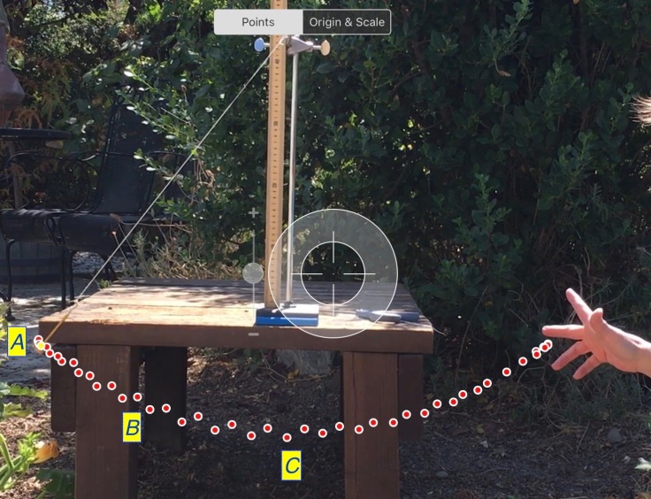
The top graph below shows the horizontal, x (red), and vertical, y (blue), positions as a function of time. The bottom graph shows the velocities in the x (red) and y (blue) directions. I marked the location of points A, B and C on the graph – again you can see at point A that the velocities are zero and the positions are at their maximum/minimum values and at point C the positions are both zero but the velocity in the x direction is at its maximum.  The velocity in the y or vertical direction is also zero at point C because the pendulum bob is really only moving horizontally at that moment. At point B, and you can pick any point between A and C, the pendulum has both potential and kinetic energies.

In the graphical analysis app you can click on a data point and the app shows you the values – those are the numbers in the white boxes. This is handy when trying to read values off the graph, especially when the app doesn’t label the tick marks.

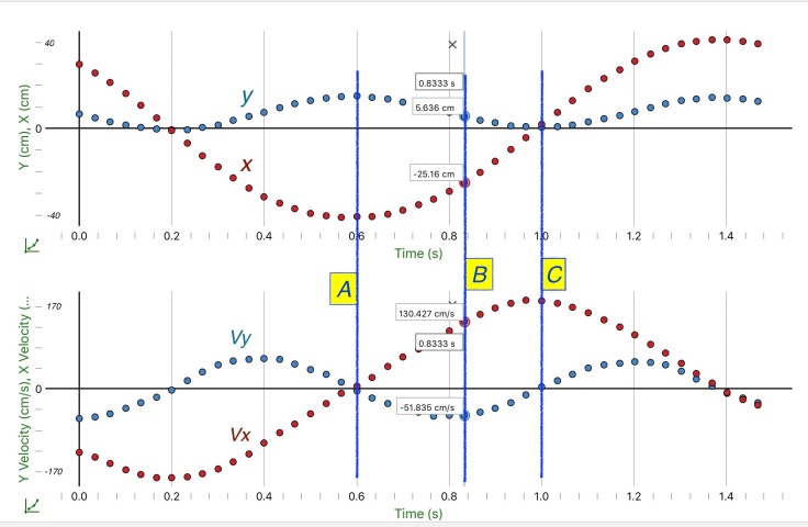
Students made a table in their lab books and recorded the height (y) of the pendulum at the three points, as well as the velocities (x & y).  Then they calculated the potential energy at each point (mgh) and the kinetic energy (1/2 m v²), m = mass of the pendulum bob which was 0.05 kg.  Finally they calculated the total energy (PE + KE) at each point and hopefully found the numbers to be roughly the same.  For the data shown above we got 0.074J for the total energy at each point.

This is a nice lab but the students get really confused looking at the graphs and confusing position for velocity, x for y, etc.  Another problem that popped up in a couple of groups was students didn’t put the origin at the bottom of the swing (C),  so when the pendulum was at C the graph showed a nonzero y-position.  You also need to make sure you mark enough points (Video Physics app)  to catch the pendulum turning around (A) and coming back through the lowest point (C).

Without even doing any math, but just looking at the graphs and realizing that the data for the height of the pendulum, y (blue dots), is proportional to the PE, reaches its maximum at the same time the velocities, and therefore KE, both go to zero.  As the horizontal velocity (red data in bottom graph) reaches its maximum value, and therefore KE will be its maximum, you can see the height (and therefore PE)  is also zero.  As one goes up the other goes down.  I guess one way to simple the graphs would have been to have them just plot vertical position (y) and horizontal velocity as a function of time and just do points A and C.  Something to think about the next time I do this lab.

I asked the students to watch these videos before class.